|
isce3
0.1.0
|
|
isce3
0.1.0
|
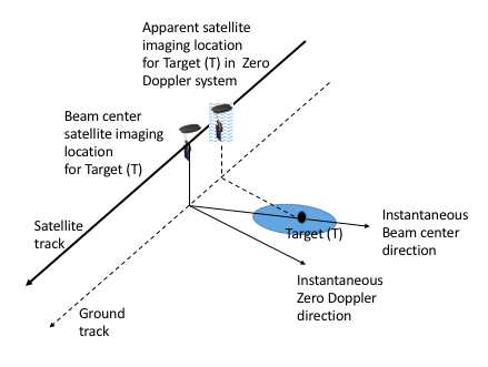
SAR focusing techniques combine information from numerous transmitted pulses to produce a high-resolution two-dimensional backscatter image of the area illuminated by the antenna footprint (see Figure below). Consequently, the observed amplitude and phase measurement at any single pixel in a SAR image cannot be attributed to any individual pulse in azimuth time or range bin in slant range. To better geolocate targets in focused SAR images, most processing approaches use various conventions based on the Range-Doppler equation to set up reference functions for compressing energy in slant range and azimuth time domains.
The Range-Doppler equation establishes the relationship between the Target T located at position ( \(\mathbf{T}\)) and the satellite imaging location:
\[ \frac{2 \cdot \mathbf{V_{sat}}\left( \eta_{f,T} \right) \cdot \left( \mathbf{T} - \mathbf{R_{sat}}\left(\eta_{f,T}\right) \right)}{\lambda \cdot R_{f,T}} = f\left(\eta_{f,T}, R_{f,T}\right) \]
\[ R_{f,T} = \left|\mathbf{T} - \mathbf{R_{sat}}\left(\eta_{f,T} \right)\right| \]
where
For a given Doppler frequency model \(f\left(\eta_{f,T},R_{f,T}\right)\), the Target T would show up at azimuth line location \( \eta_{f,T}\) and slant range location \(R_{f,T}\) in the focused image. Note that the choice of Doppler frequency model to describe the geometry of the SAR image can be arbitrary. However, there are two standard conventions widely used for easy interpretation of the imaging geometry: Native Doppler (or Beam Center) geometry and the Zero Doppler (or Tangential) geometry. ISCE supports both these conventions.
The Native Doppler geometry system is the most natural system for representing SAR data. In this case, the Doppler frequency model is chosen to match the estimated Doppler Centroid of the data, i.e.:
\[ \frac{2 \cdot \mathbf{V_{sat}}\left( \eta_{dc,T} \right) \cdot \left( \mathbf{T} - \mathbf{R_{sat}}\left(\eta_{dc,T}\right) \right)}{\lambda \cdot R_{dc,T}} = f\left(\eta_{dc,T}, R_{dc,T}\right) \]
The Doppler Centroid at a given azimuth time and slant range determines the imaging geometry as well as the azimuth carrier on the data. The azimuth time and slant range correspond to the target’s passage through the center of the antenna along track footprint. The Native Doppler convention is ideal for applying antenna pattern and gain corrections. However, the Doppler Centroid of the acquired data can vary in both azimuth time and slant range. Consequently, patch processing of the SAR pulses that accounts for updated processing parameter along-track introduces complications. The dependence on Doppler Centroid also makes it a little more complicated to mosaic acquisitions on the same track that were processed with slightly different processing parameters.
The Native Doppler convention is primarily used by NASA JPL for generating SAR imagery for its airborne missions like UAVSAR. The ALOS PALSAR L1.1 product was also produced in Native Doppler geometry system by JAXA.
The Zero Doppler geometry system is the most widely used convention for representing SAR data. In this case, Doppler frequency model is set to zero, i.e.:
\[ \mathbf{V_{sat}}\left( \eta_{0,T} \right) \cdot \left( \mathbf{T} - \mathbf{R_{sat}}\left(\eta_{0,T}\right) \right) = 0 \]
The imaging geometry can be determined independent of the Doppler Centroid and central frequency of the acquisition. The vector from the satellite to target is perpendicular to the instantaneous satellite velocity. Note that in case of the zero Doppler geometry, the azimuth time corresponding to a target can lie outside the interval defined by the imaging aperture. The SAR data still has an azimuth carrier defined by the Doppler Centroid but this piece of information does not affect the geolocation or interpretation of the imaging geometry. This independence between Doppler Centroid and imaging geometry, allows one to mosaic images on the same track processed with different parameters easily.
The Zero Doppler convention is used by ESA and European sensors like ERS, ENVISAT ([3], [13]), Sentinel-1 [10] as well as TerraSAR-X and COSMO-SkyMed. The ALOS-2 PALSAR L1.1 product is also produced in Zero Doppler geometry system by JAXA.
The forward geometry transformation is implemented via isce3::geometry::Topo module in ISCE.
This algorithm maps a given Target (T) located at azimuth time \( \left( \eta_{dc,T} \right) \) and slant range \(\left( R_{dc,T}\right) \) in radar image coordinates to map coordinates \(\left(X_{map}, Y_{map}, h\left(X_{map}, Y_{map}\right)\right)\). This is done using the given Doppler model \(\left( f_d\left(\eta,R\right)\right)\) and a Digital Elevation Model (DEM) \( \left(z\left( X, Y\right)\right)\) as function of horizontal datum coordinates X, Y. Details of various implementations of the forward mapping algorithm can be found in a number of references ([7], [2], [12], [9]).
The forward mapping problem is formulated as finding target position \(\mathbf{T}\), such that the following two constraints are satisfied
\[ \frac{2 \mathbf{V_{sat}\left(\eta_{dc,T}\right)} \cdot \left( \mathbf{T} - \mathbf{R_{sat}\left(\eta_{dc,T}\right)} \right)}{\lambda \cdot R_{dc,T}} = f_{dc}\left(\eta_{dc,T}, R_{dc,T} \right) \]
\[ \left| \mathbf{T} - \mathbf{R_{sat}\left(\eta_{dc,T}\right)} \right | = R_{dc,T} \]
In ISCE, the algorithm is broken down into 4 steps. Note that all computations are performed in the Earth Centered Earth Fixed (ECEF) coordinates.
Setting up of a local Geocentric spherical coordinate system at the location of the satellite. Initializing the height of the target above local sphere to a nominal value \(h_p\).
Solve the constrained optimization problem shown above for point \(\mathbf{T}\) on the local sphere. Convert the location of the coordinates to map coordinates - \(X_{map}, Y_{map}\). Note that only the horizontal location information is used from this estimate for the next stage of the algorithm.
Interpolate the given DEM \( z\left(X,Y\right) \) to obtain \(z_{map}\). Conver the coordinates \(\left(X_{map}, Y_{map}, z_{map}\right)\) to the local spherical system and estimate the height above the local sphere \(h_{est}\).
Each of the steps is described in detail below. The algorithm can support analysis in both Native Doppler and Zero Doppler coordinate systems. For Zero Doppler coordinate system, the Doppler model \( \left( f_{d}\left(\eta_{dc,T}, R_{dc,T}\right) \right) \) is set to zero.
Let \(\mathbf{R_{sat}}\) and \(\mathbf{V_{sat}}\) represent the position of the satellite corresponding to the azimuth time of the target of interest. The Geocentric radius at the intersection of the reference Ellipsoid and the vector connecting the satellite position to the center of the Ellipsoid is given by
\[ R_c =\frac{\left| \mathbf{R_{sat}}\right|} {\sqrt{ \left( \frac{X_{sat}}{a_e} \right)^2 + \left( \frac{Y_{sat}}{a_e} \right)^2 + \left( \frac{Z_{sat}}{b_e} \right)^2 }} \]
Relative height of the satellite along the Geocentric vector is given by
\[ h_{sat} = \left| \mathbf{R_{sat}} \right| - R_c \]
We can set up a local orthogonal coordinate system on a sphere with radius \(R_c\) at \(\mathbf{R_{sat}}\) as follows:
\[ \hat{n} = -\left[ \frac{X_{sat}}{\left| \mathbf{R_{sat}} \right|}, \frac{Y_{sat}}{\left| \mathbf{R_{sat}} \right|}, \frac{Z_{sat}}{\left| \mathbf{R_{sat}} \right|} \right] \]
\[ \hat{c} = \frac{\mathbf{V_{sat}} \times \hat{n}}{\left| \mathbf{V_{sat}} \times \hat{n} \right| } \]
\[ \hat{t} = \hat{c} \times \hat{n} \]
where
Assuming that the target point is located at height \(h_0\) above the local sphere of radius ( \(R_c\)), the slant range vector of length \(R_0\) can be represented in the local TCN basis as
\[ \mathbf{T} = \mathbf{R_{sat}} + \alpha \cdot \hat{t} + \beta \cdot \hat{c} + \gamma \cdot \hat{n} \]
Using the law of cosines on the local sphere, we can show that
\[ \gamma = \frac{R_0}{2} \cdot \left[ \left( \frac{h_{sat} + R_c}{R_0}\right) + \left( \frac{R_0}{h_{sat} + R_c } \right) - \left( \frac{h_0 + R_c}{h_{sat}+R_c} \right) \cdot \left( \frac{h_0 + R_{curv}}{R_0} \right) \right] \]
\[ \alpha = \frac{f_d\left(R_0\right) \cdot \lambda \cdot R_0}{2 \cdot \left| \mathbf{V_{sat}} \right|} - \gamma \cdot \frac{\hat{n} \cdot \hat{v}}{\hat{t} \cdot \hat{v}} \]
where \(\hat{v} = \frac{\mathbf{V_{sat}}}{\left| \mathbf{V_{sat}} \right|}\) is the unit vector along the satellite velocity.
\[ \beta = -L\cdot \sqrt{R_0^2 - \gamma^2 - \alpha^2} \]
where \(L=-1\) for right looking imaging geometry and \(L=+1\) for left looking imaging geometry. Once \( \alpha, \beta\) and \(\gamma\) are computd, we can compute the location of the target in Cartesian space \(\left( \mathbf{T} \right)\). The target location can be converted into map coordinates as \(\left( X_{map}, Y_{map}, z_map\left(X_{map}, Y_{map}\right) \right)\) using standard transformations (see isce3::core::ProjectionBase).
DEMs are commonly provided in non-Cartesian coordinates (e.g., Lat-Long grid, UTM grid, EASE-2 grid) and contain heights above a geoid (e.g., EGM96 or EGM08). The geometry mapping algorithms presented in this document explicitly assume that the DEMs have been adjusted to represent heights above the representative ellipsoid like WGS84. Standard GIS tools offer numerous methods of interpolating height data (e.g., nearest neighbor, bilinear, and bicubic). We recommend using biquintic interpolation method [5] as this appears to be least susceptible to difference between the DEM resolution and the radar grid resolution to which it is being mapped. Moreover, biquintic polynomials represent the smallest order polynomials that preserve slope information when interpolating across neighboring cells in the DEM.
For the forward mapping algorithm, we interpolate the DEM at location \(\left(X_{map}, Y_{map}\right)\) to determine the new \(z_{map}\). This new target location is then transformed into the ECEF coordinate system and the new height estimate \(h_est\) is given by
\[ h_{est} = \left| \mathbf{T} \right| - R_c \]
and \(h_{est}\) becomes the initial height estimate \(h_0\) for the next iteration of the algorithm. When trying to estimate the target location on a reference ellipsoid, the DEM is assumed to be of constant height \(z_{map}\) and the algorithm converges in two or three iterations.
This algorithm maps a given target ( \(\mathbf{T}\)) located at \(\left (X,Y, z\left(X,Y\right)\right)\) in map coordinates represented by horizontal datum \(\left(X,Y\right)\) to radar images coordinates - azimuth time ( \(\eta\)) and slant range ( \(R\)), using a given Doppler model \(\left(f_d \left(\eta,R\right)\right)\). Different implementations of the Inverse Mapping Algorithm can be found in several references ([2], [12], [9]).
The ISCE implementation of the algorithm is based on the simple Newton-Raphson method and has three key steps:
Each of the steps is described in detail below. The algorithm can support analysis in both Native Doppler and Zero Doppler coordinate systems. For Zero Doppler coordinate system, the Doppler model \(\left( f_d\left(\eta_{dc,T}, R_{dc,T}\right)\right)\) is set to zero.
To precisely map targets from map coordinates to radar image coordinaes, we need to be able to interpolate the orbit state vectors with an accuracy on order of few mm. Two possible interpolation methods satisfy this requirement:
Hermite polynomial interpolation
A third-order Hermite polynomial can be used to interpolate the orbit information reliably. The Hermite polynomial is constructed using 4 state vectors spanning the azimuth time epoch of interest; and combines position and velocity information for interpolating the state vectors [11]. Hermite polynomials works better in the scenario when the available state vectors are sampled less frequently than once every 30 seconds.
For most modern SAR sensors, the precise position and velocity vectors in the annotation metadata are consistent with each other and can be reliably interpolated with Hermite polynomials. However, when focusing the L0B data for emergency response, the precise state vectors may not be available. Legendre polynomials are recommended for interpolation of the rapid orbits as it reduces geolocation errors.
At the start of the algorithm, we pick and initial azimuth time ( \(\eta_g\)) as the first guess. Typically, this is set to the center of the azimuth data block / scene that is being processed. After interpolation, we end up with the initial estimate for satellite position \(\left( \mathbf{R_{sat}\left( \eta_g \right)} \right)\) and satellite velocity \(\left( \mathbf{V_{sat}\left( \eta_g \right)} \right)\).
The function \(y\left( \eta \right)\), whose zero crossing we are trying to determine using the Newton-Raphson method can be directly derived from the Range Doppler Equation.
\[ y\left( \eta \right) = \mathbf{V_{sat}\left(\eta\right)} \cdot \left( \mathbf{T} - \mathbf{R_{sat}\left( \eta \right)}\right) - \frac{\lambda}{2} \cdot f_d\left( \eta, R_{dc}\left(\eta\right)\right) \cdot R_dc\left( \eta \right) = 0 \]
where
\[ R_{dc}\left(\eta \right) = \left| \mathbf{T} - \mathbf{R_{sat}\left(\eta\right)}\right| \]
The adjustment to the initial guess of the azimuth time epoch ( \(\eta_g\)) is given by
\[ \eta_{new} = \eta_g - \frac{y\left( \eta_g \right)}{y^{\prime}\left( \eta_g\right)} \]
where
\[ y^{\prime}\left( \eta \right) \approx \frac{\lambda}{2} \cdot \left[ \frac{ f_{dc}\left( \eta, R_{dc}\left( \eta \right) \right)}{R_{dc}\left( \eta \right)} + f_d^{\prime}\left( \eta, R_{dc}\left( \eta \right) \right) \right] \cdot \left( \mathbf{V_{sat}\left( \eta \right)} \cdot \left( \mathbf{T} - \mathbf{R_{sat}\left(\eta\right)} \right) - \left| \mathbf{V_{sat}\left( \eta \right)}\right|^2 \right) \]
The Newton-Raphson iterations are continued till the estimated azimuth time converges, i.e, the Range-Doppler equation is satisfied. When the algorithm converges \(R_{dc}\left( \eta_{new} \right)\) represents the slant range to the target.
 1.8.5.

